Flu Analysis: Fitting

Load the data and packages:

library(tidyverse)
Warning: package 'tidyverse' was built under R version 4.2.2
── Attaching packages ─────────────────────────────────────── tidyverse 1.3.2 ──
✔ ggplot2 3.4.0      ✔ purrr   1.0.1 
✔ tibble  3.1.8      ✔ dplyr   1.0.10
✔ tidyr   1.2.1      ✔ stringr 1.5.0 
✔ readr   2.1.3      ✔ forcats 0.5.2 
Warning: package 'ggplot2' was built under R version 4.2.2
Warning: package 'stringr' was built under R version 4.2.2
── Conflicts ────────────────────────────────────────── tidyverse_conflicts() ──
✖ dplyr::filter() masks stats::filter()
✖ dplyr::lag()    masks stats::lag()
library(tidymodels) #build models
Warning: package 'tidymodels' was built under R version 4.2.2
── Attaching packages ────────────────────────────────────── tidymodels 1.0.0 ──
✔ broom        1.0.3     ✔ rsample      1.1.1
✔ dials        1.1.0     ✔ tune         1.0.1
✔ infer        1.0.4     ✔ workflows    1.1.2
✔ modeldata    1.1.0     ✔ workflowsets 1.0.0
✔ parsnip      1.0.3     ✔ yardstick    1.1.0
✔ recipes      1.0.4     
Warning: package 'broom' was built under R version 4.2.2
Warning: package 'dials' was built under R version 4.2.2
Warning: package 'infer' was built under R version 4.2.2
Warning: package 'modeldata' was built under R version 4.2.2
Warning: package 'parsnip' was built under R version 4.2.2
Warning: package 'recipes' was built under R version 4.2.2
Warning: package 'rsample' was built under R version 4.2.2
Warning: package 'tune' was built under R version 4.2.2
Warning: package 'workflows' was built under R version 4.2.2
Warning: package 'workflowsets' was built under R version 4.2.2
Warning: package 'yardstick' was built under R version 4.2.2
── Conflicts ───────────────────────────────────────── tidymodels_conflicts() ──
✖ scales::discard() masks purrr::discard()
✖ dplyr::filter()   masks stats::filter()
✖ recipes::fixed()  masks stringr::fixed()
✖ dplyr::lag()      masks stats::lag()
✖ yardstick::spec() masks readr::spec()
✖ recipes::step()   masks stats::step()
• Use suppressPackageStartupMessages() to eliminate package startup messages
library(here) #help read/import data
Warning: package 'here' was built under R version 4.2.2
here() starts at C:/Users/Raquel/GitHub/MADA/RaquelFrancisco-MADA-portfolio
library(ggplot2) #data visualization
library(broom.mixed) # for converting bayesian models to tidy tibbles
Warning: package 'broom.mixed' was built under R version 4.2.2
library(dotwhisker)  # for visualizing regression results
Warning: package 'dotwhisker' was built under R version 4.2.2
library(performance) #evaluate model fit and performance
Warning: package 'performance' was built under R version 4.2.2

Attaching package: 'performance'

The following objects are masked from 'package:yardstick':

    mae, rmse
data <- readRDS(here('fluanalysis/data/SypAct_clean.rds')) #upload cleaned data
tibble(data) # to get a look at the data
# A tibble: 730 × 26
   SwollenLymph…¹ Chest…² Chill…³ Nasal…⁴ Sneeze Fatigue Subje…⁵ Heada…⁶ Weakn…⁷
   <fct>          <fct>   <fct>   <fct>   <fct>  <fct>   <fct>   <fct>   <fct>  
 1 Yes            No      No      No      No     Yes     Yes     Yes     Mild   
 2 Yes            Yes     No      Yes     No     Yes     Yes     Yes     Severe 
 3 Yes            Yes     Yes     Yes     Yes    Yes     Yes     Yes     Severe 
 4 Yes            Yes     Yes     Yes     Yes    Yes     Yes     Yes     Severe 
 5 Yes            No      Yes     No      No     Yes     Yes     Yes     Modera…
 6 No             No      Yes     No      Yes    Yes     Yes     Yes     Modera…
 7 No             No      Yes     No      No     Yes     Yes     No      Mild   
 8 No             Yes     Yes     Yes     Yes    Yes     Yes     Yes     Severe 
 9 Yes            Yes     Yes     Yes     No     Yes     Yes     Yes     Modera…
10 No             Yes     No      Yes     No     Yes     No      Yes     Modera…
# … with 720 more rows, 17 more variables: CoughIntensity <fct>, Myalgia <fct>,
#   RunnyNose <fct>, AbPain <fct>, ChestPain <fct>, Diarrhea <fct>,
#   EyePn <fct>, Insomnia <fct>, ItchyEye <fct>, Nausea <fct>, EarPn <fct>,
#   Pharyngitis <fct>, Breathless <fct>, ToothPn <fct>, Vomit <fct>,
#   Wheeze <fct>, BodyTemp <dbl>, and abbreviated variable names
#   ¹​SwollenLymphNodes, ²​ChestCongestion, ³​ChillsSweats, ⁴​NasalCongestion,
#   ⁵​SubjectiveFever, ⁶​Headache, ⁷​Weakness
str(data)
'data.frame':   730 obs. of  26 variables:
 $ SwollenLymphNodes: Factor w/ 2 levels "No","Yes": 2 2 2 2 2 1 1 1 2 1 ...
  ..- attr(*, "label")= chr "Swollen Lymph Nodes"
 $ ChestCongestion  : Factor w/ 2 levels "No","Yes": 1 2 2 2 1 1 1 2 2 2 ...
  ..- attr(*, "label")= chr "Chest Congestion"
 $ ChillsSweats     : Factor w/ 2 levels "No","Yes": 1 1 2 2 2 2 2 2 2 1 ...
  ..- attr(*, "label")= chr "Chills/Sweats"
 $ NasalCongestion  : Factor w/ 2 levels "No","Yes": 1 2 2 2 1 1 1 2 2 2 ...
  ..- attr(*, "label")= chr "Nasal Congestion"
 $ Sneeze           : Factor w/ 2 levels "No","Yes": 1 1 2 2 1 2 1 2 1 1 ...
  ..- attr(*, "label")= chr "Sneeze"
 $ Fatigue          : Factor w/ 2 levels "No","Yes": 2 2 2 2 2 2 2 2 2 2 ...
  ..- attr(*, "label")= chr "Fatigue"
 $ SubjectiveFever  : Factor w/ 2 levels "No","Yes": 2 2 2 2 2 2 2 2 2 1 ...
  ..- attr(*, "label")= chr "Subjective Fever"
 $ Headache         : Factor w/ 2 levels "No","Yes": 2 2 2 2 2 2 1 2 2 2 ...
  ..- attr(*, "label")= chr "Headache"
 $ Weakness         : Factor w/ 4 levels "None","Mild",..: 2 4 4 4 3 3 2 4 3 3 ...
 $ CoughIntensity   : Factor w/ 4 levels "None","Mild",..: 4 4 2 3 1 3 4 3 3 3 ...
  ..- attr(*, "label")= chr "Cough Severity"
 $ Myalgia          : Factor w/ 4 levels "None","Mild",..: 2 4 4 4 2 3 2 4 3 2 ...
 $ RunnyNose        : Factor w/ 2 levels "No","Yes": 1 1 2 2 1 1 2 2 2 2 ...
  ..- attr(*, "label")= chr "Runny Nose"
 $ AbPain           : Factor w/ 2 levels "No","Yes": 1 1 2 1 1 1 1 1 1 1 ...
  ..- attr(*, "label")= chr "Abdominal Pain"
 $ ChestPain        : Factor w/ 2 levels "No","Yes": 1 1 2 1 1 2 2 1 1 1 ...
  ..- attr(*, "label")= chr "Chest Pain"
 $ Diarrhea         : Factor w/ 2 levels "No","Yes": 1 1 1 1 1 2 1 1 1 1 ...
 $ EyePn            : Factor w/ 2 levels "No","Yes": 1 1 1 1 2 1 1 1 1 1 ...
  ..- attr(*, "label")= chr "Eye Pain"
 $ Insomnia         : Factor w/ 2 levels "No","Yes": 1 1 2 2 2 1 1 2 2 2 ...
  ..- attr(*, "label")= chr "Sleeplessness"
 $ ItchyEye         : Factor w/ 2 levels "No","Yes": 1 1 1 1 1 1 1 1 1 1 ...
  ..- attr(*, "label")= chr "Itchy Eyes"
 $ Nausea           : Factor w/ 2 levels "No","Yes": 1 1 2 2 2 2 1 1 2 2 ...
 $ EarPn            : Factor w/ 2 levels "No","Yes": 1 2 1 2 1 1 1 1 1 1 ...
  ..- attr(*, "label")= chr "Ear Pain"
 $ Pharyngitis      : Factor w/ 2 levels "No","Yes": 2 2 2 2 2 2 2 1 1 1 ...
  ..- attr(*, "label")= chr "Sore Throat"
 $ Breathless       : Factor w/ 2 levels "No","Yes": 1 1 2 1 1 2 1 1 1 2 ...
  ..- attr(*, "label")= chr "Breathlessness"
 $ ToothPn          : Factor w/ 2 levels "No","Yes": 1 1 2 1 1 1 1 1 2 1 ...
  ..- attr(*, "label")= chr "Tooth Pain"
 $ Vomit            : Factor w/ 2 levels "No","Yes": 1 1 1 1 1 1 2 1 1 1 ...
  ..- attr(*, "label")= chr "Vomiting"
 $ Wheeze           : Factor w/ 2 levels "No","Yes": 1 1 1 2 1 2 1 1 1 1 ...
  ..- attr(*, "label")= chr "Wheezing"
 $ BodyTemp         : num  98.3 100.4 100.8 98.8 100.5 ...
Code will include:

  • Fitting a linear model to the continuous outcome (Body temperature) using only the main predictor of interest.

  • Fitting another linear model to the continuous outcome using all (important) predictors of interest.

  • Comparing the model results for the model with just the main predictor and all predictors.

  • Fitting a logistic model to the categorical outcome (Nausea) using only the main predictor of interest.

  • Fitting another logistic model to the categorical outcome using all (important) predictors of interest.

  • Compares the model results for the categorical model with just the main predictor and all predictors.

Linear Model: Body Temperature vs. Myalgia

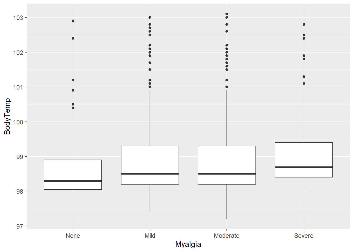
#plot suspect interaction
ggplot(data,
       aes(x = Myalgia, y = BodyTemp)) + 
  geom_boxplot()

lm_mod <- linear_reg() #note the default is lm(), thus we do not need to "set" the computational engine

lm_fit1 <- lm_mod %>% 
  fit(BodyTemp ~ Myalgia, data = data)

tidy(lm_fit1) #several significant results
# A tibble: 4 × 5
  term            estimate std.error statistic p.value
  <chr>              <dbl>     <dbl>     <dbl>   <dbl>
1 (Intercept)       98.7       0.134    734.    0     
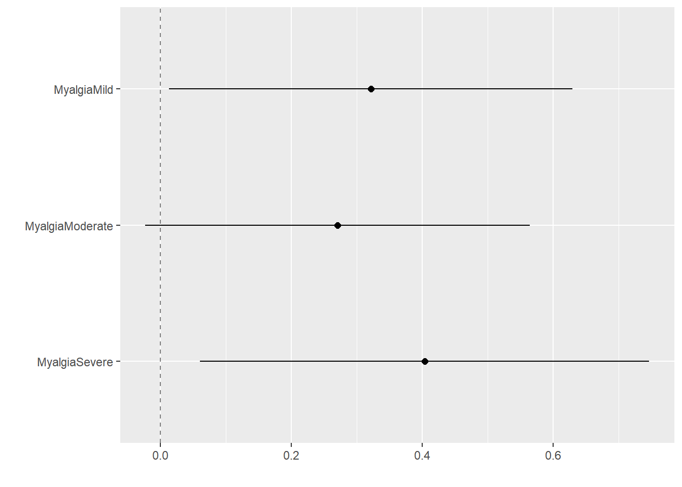
2 MyalgiaMild        0.322     0.157      2.04  0.0413
3 MyalgiaModerate    0.271     0.150      1.81  0.0711
4 MyalgiaSevere      0.404     0.175      2.31  0.0214
tidy(lm_fit1) %>% ##help visualize model with dot-whisker plot
  dwplot(dot_args = list(size = 2, color = "black"),
         whisker_args = list(color = "black"),
         vline = geom_vline(xintercept = 0, colour = "grey50", linetype = 2))

Linear Model: Body Temperature vs. All Variables

lm_fit_all1 <- lm_mod %>% 
  fit(BodyTemp ~ ., data = data)

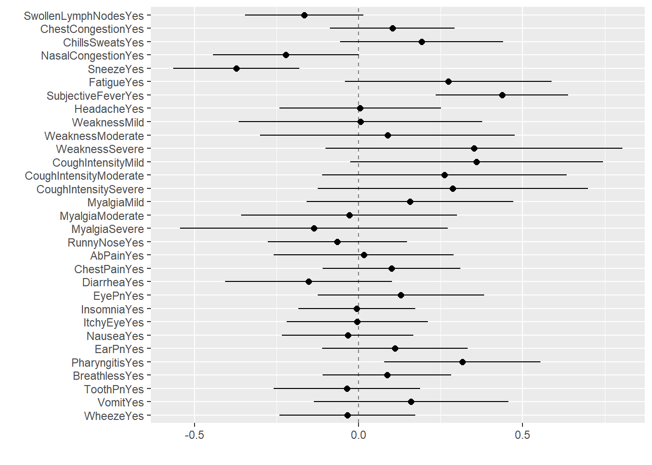
tidy(lm_fit_all1) #several significant results
# A tibble: 32 × 5
   term                 estimate std.error statistic   p.value
   <chr>                   <dbl>     <dbl>     <dbl>     <dbl>
 1 (Intercept)          97.9        0.304   323.     0        
 2 SwollenLymphNodesYes -0.166      0.0920   -1.81   0.0714   
 3 ChestCongestionYes    0.103      0.0971    1.06   0.291    
 4 ChillsSweatsYes       0.192      0.127     1.51   0.131    
 5 NasalCongestionYes   -0.222      0.113    -1.95   0.0512   
 6 SneezeYes            -0.373      0.0980   -3.80   0.000156 
 7 FatigueYes            0.273      0.161     1.70   0.0901   
 8 SubjectiveFeverYes    0.437      0.103     4.25   0.0000244
 9 HeadacheYes           0.00498    0.125     0.0397 0.968    
10 WeaknessMild          0.00552    0.189     0.0292 0.977    
# … with 22 more rows
tidy(lm_fit_all1) %>% ##help visualize regression with dot-whisker plot w/ 95% CI
  dwplot(dot_args = list(size = 2, color = "black"), #Coefficient Estimates
         whisker_args = list(color = "black"), #CI
         vline = geom_vline(xintercept = 0, colour = "grey50", linetype = 2))

Model Output Comparison

#Check the goodness of "fit" with these 2 lm() models
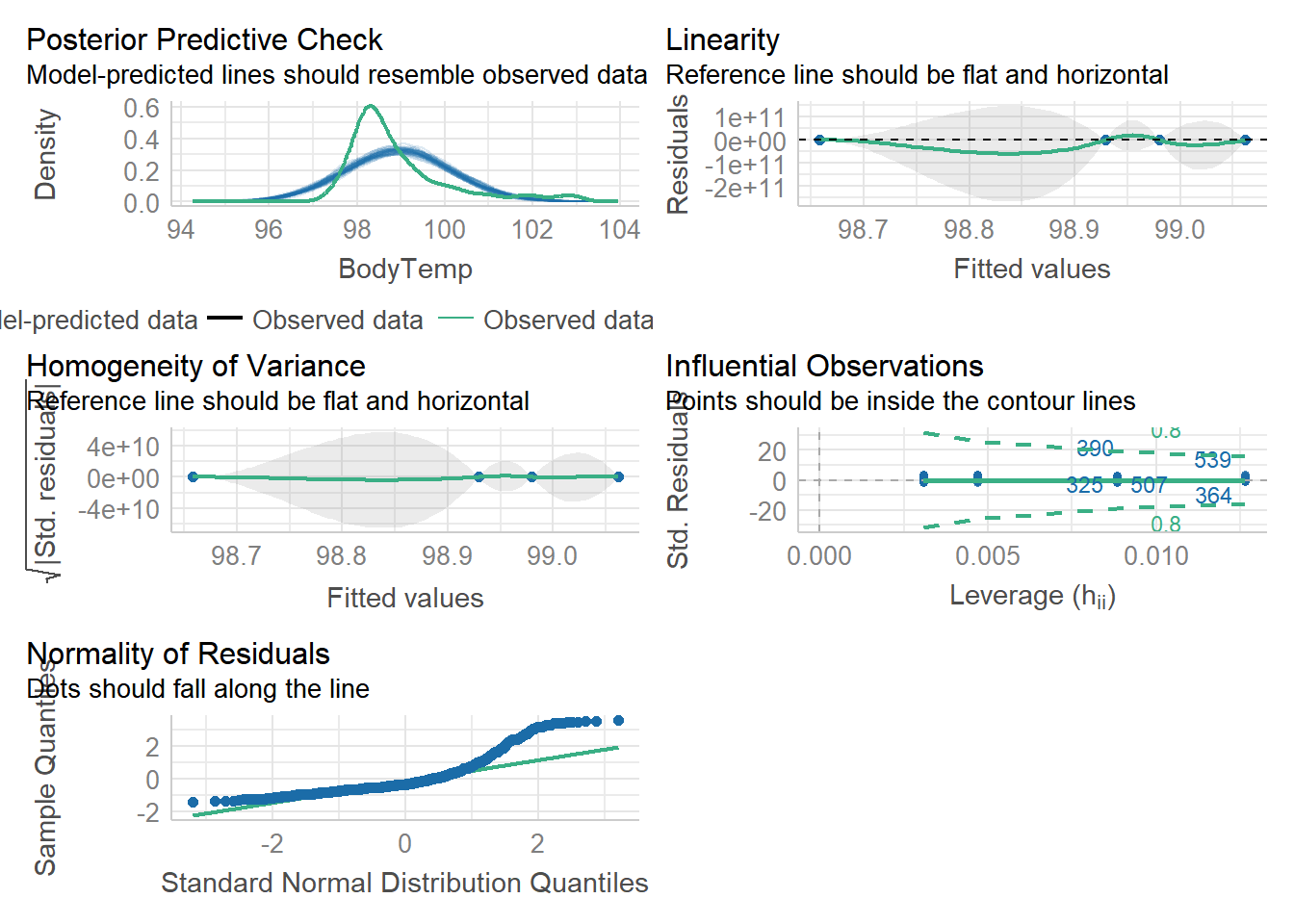
check_model(lm_fit1$fit) #allows for streamlined way to look at QQ plot, normality, etc

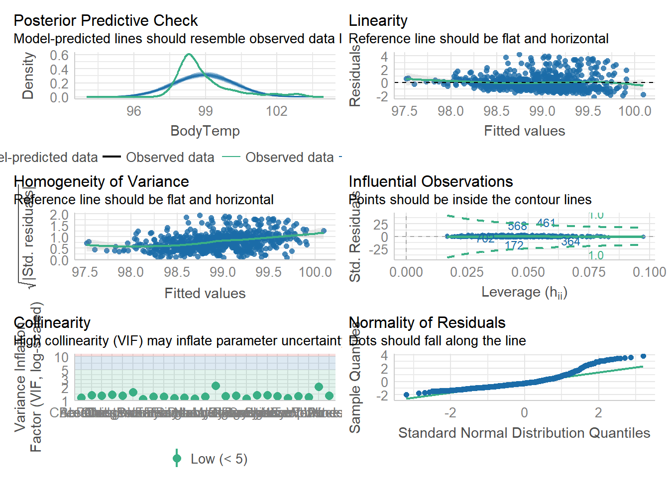
check_model(lm_fit_all1$fit)
Variable `Component` is not in your data frame :/

#Compare output
#Visually
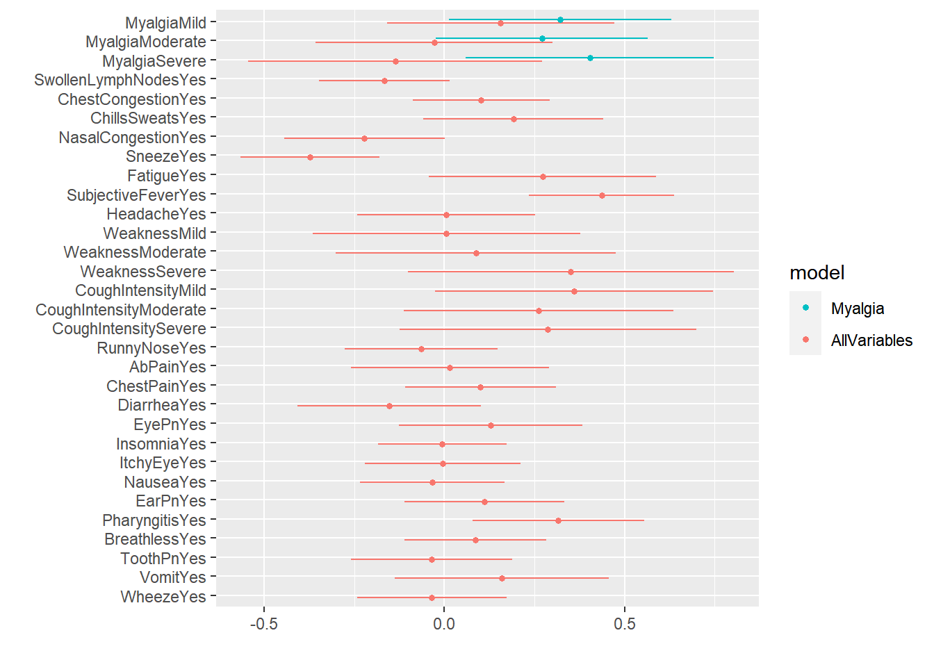
dwplot(list(Myalgia = lm_fit1, AllVariables = lm_fit_all1)) #compare dwplots

glance(lm_fit1) %>%
  dplyr::select(adj.r.squared, AIC, BIC, p.value)
# A tibble: 1 × 4
  adj.r.squared   AIC   BIC p.value
          <dbl> <dbl> <dbl>   <dbl>
1       0.00387 2337. 2360.   0.121
glance(lm_fit_all1) %>%
  dplyr::select(adj.r.squared, AIC, BIC, p.value)
# A tibble: 1 × 4
  adj.r.squared   AIC   BIC      p.value
          <dbl> <dbl> <dbl>        <dbl>
1        0.0853 2302. 2453. 0.0000000247
compare_performance(lm_fit1,lm_fit_all1) #better way
# Comparison of Model Performance Indices

Name        | Model |  AIC (weights) | AICc (weights) |  BIC (weights) |    R2 | R2 (adj.) |  RMSE | Sigma
----------------------------------------------------------------------------------------------------------
lm_fit1     |   _lm | 2336.6 (<.001) | 2336.6 (<.001) | 2359.5 (>.999) | 0.008 |     0.004 | 1.191 | 1.194
lm_fit_all1 |   _lm | 2301.6 (>.999) | 2304.8 (>.999) | 2453.1 (<.001) | 0.124 |     0.085 | 1.119 | 1.144
#Via ANOVA
anova(lm_fit1$fit, lm_fit_all1$fit)
Analysis of Variance Table

Model 1: BodyTemp ~ Myalgia
Model 2: BodyTemp ~ SwollenLymphNodes + ChestCongestion + ChillsSweats + 
    NasalCongestion + Sneeze + Fatigue + SubjectiveFever + Headache + 
    Weakness + CoughIntensity + Myalgia + RunnyNose + AbPain + 
    ChestPain + Diarrhea + EyePn + Insomnia + ItchyEye + Nausea + 
    EarPn + Pharyngitis + Breathless + ToothPn + Vomit + Wheeze
  Res.Df     RSS Df Sum of Sq      F    Pr(>F)    
1    726 1035.07                                  
2    698  913.79 28    121.28 3.3086 3.294e-08 ***
---
Signif. codes:  0 '***' 0.001 '**' 0.01 '*' 0.05 '.' 0.1 ' ' 1

Logistic Model: Nausea vs. Myalgia

#plot suspect interaction
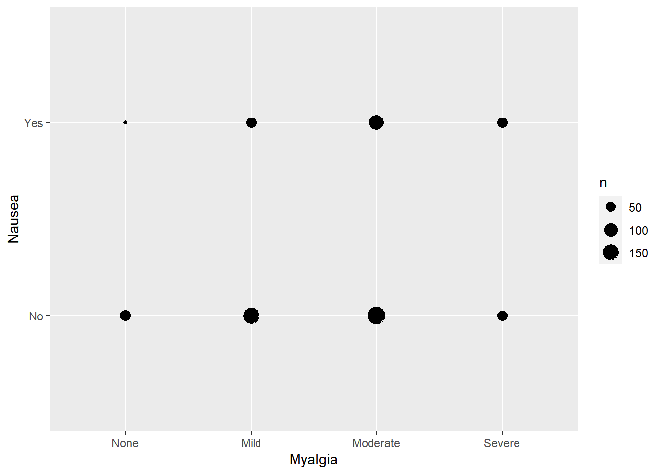
ggplot(data, aes(x = Myalgia, y = Nausea)) + 
  geom_count()

glm_mod <- logistic_reg(mode = "classification",
  engine = "glm",
  penalty = NULL,
  mixture = NULL) #define mode so it is a glm

glm_fit1 <- glm_mod %>% 
  fit(Nausea ~ Myalgia, data = data)

tidy(glm_fit1) #several significant results
# A tibble: 4 × 5
  term            estimate std.error statistic     p.value
  <chr>              <dbl>     <dbl>     <dbl>       <dbl>
1 (Intercept)       -1.37      0.280    -4.90  0.000000980
2 MyalgiaMild        0.291     0.321     0.905 0.366      
3 MyalgiaModerate    0.926     0.302     3.07  0.00217    
4 MyalgiaSevere      1.42      0.337     4.22  0.0000244  
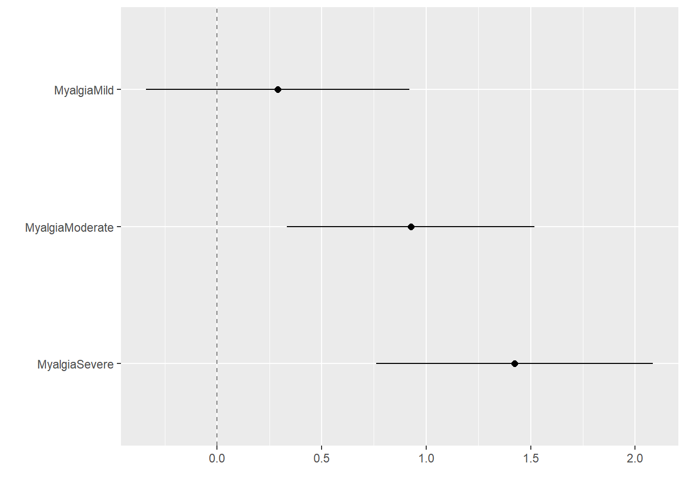
tidy(glm_fit1) %>% ##help visualize model with dot-whisker plot
  dwplot(dot_args = list(size = 2, color = "black"),
         whisker_args = list(color = "black"),
         vline = geom_vline(xintercept = 0, colour = "grey50", linetype = 2))

Logistic Model: Nausea vs. All Variables

glm_fit_all1 <- glm_mod %>% 
  fit(Nausea ~ ., data = data)

tidy(glm_fit_all1) #several significant results
# A tibble: 32 × 5
   term                 estimate std.error statistic p.value
   <chr>                   <dbl>     <dbl>     <dbl>   <dbl>
 1 (Intercept)             0.207     7.81     0.0265  0.979 
 2 SwollenLymphNodesYes   -0.247     0.196   -1.26    0.207 
 3 ChestCongestionYes      0.265     0.210    1.26    0.207 
 4 ChillsSweatsYes         0.291     0.287    1.01    0.311 
 5 NasalCongestionYes      0.440     0.253    1.74    0.0822
 6 SneezeYes               0.165     0.210    0.787   0.431 
 7 FatigueYes              0.231     0.371    0.622   0.534 
 8 SubjectiveFeverYes      0.255     0.223    1.14    0.253 
 9 HeadacheYes             0.337     0.285    1.18    0.236 
10 WeaknessMild           -0.120     0.447   -0.269   0.788 
# … with 22 more rows
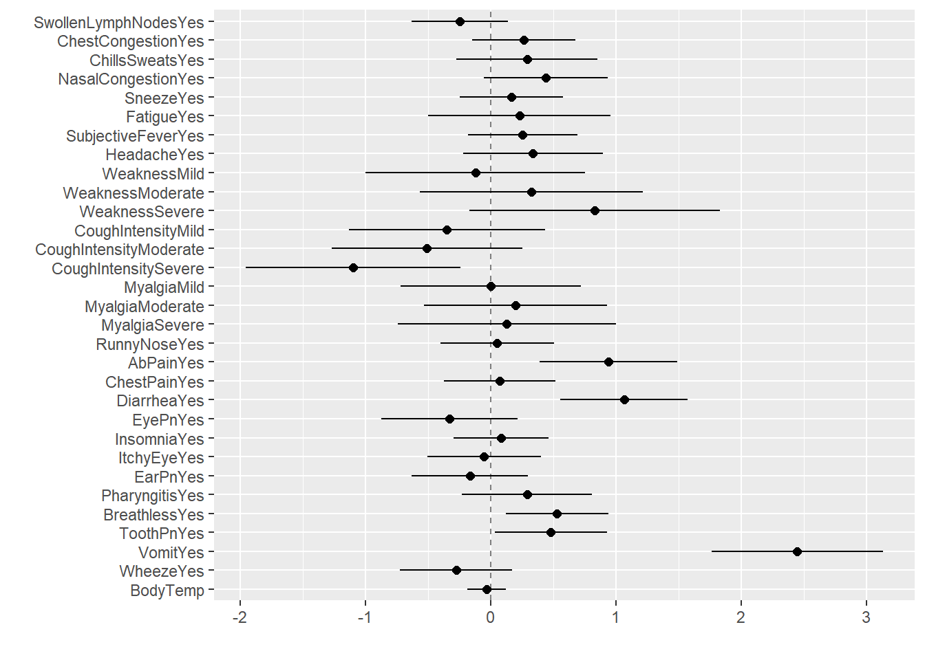
tidy(glm_fit_all1) %>% ##help visualize regression with dot-whisker plot w/ 95% CI
  dwplot(dot_args = list(size = 2, color = "black"), #Coefficient Estimates
         whisker_args = list(color = "black"), #CI
         vline = geom_vline(xintercept = 0, colour = "grey50", linetype = 2))

Model Output Comparison

#Check the goodness of "fit" with these 2 lm() models
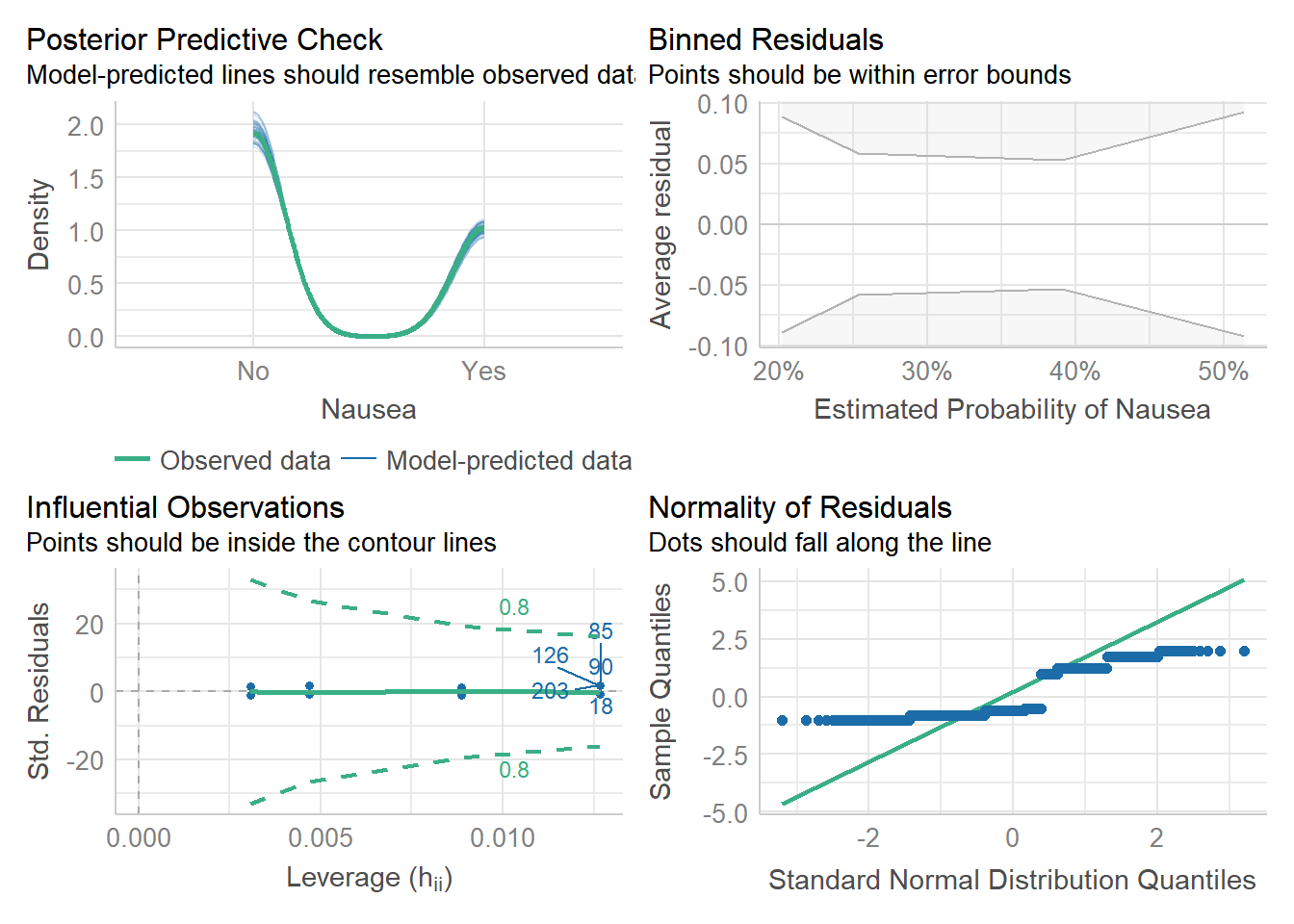
check_model(glm_fit1$fit) #QQ plot seems off, residuals may be an issue

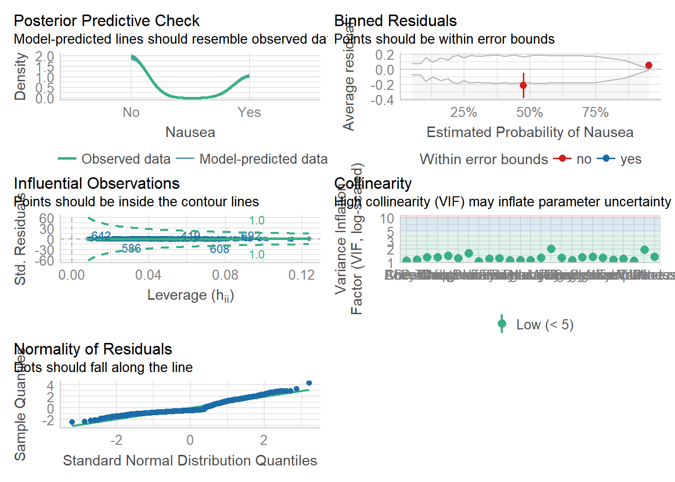
check_model(glm_fit_all1$fit)
Variable `Component` is not in your data frame :/

#Compare output
#Visually
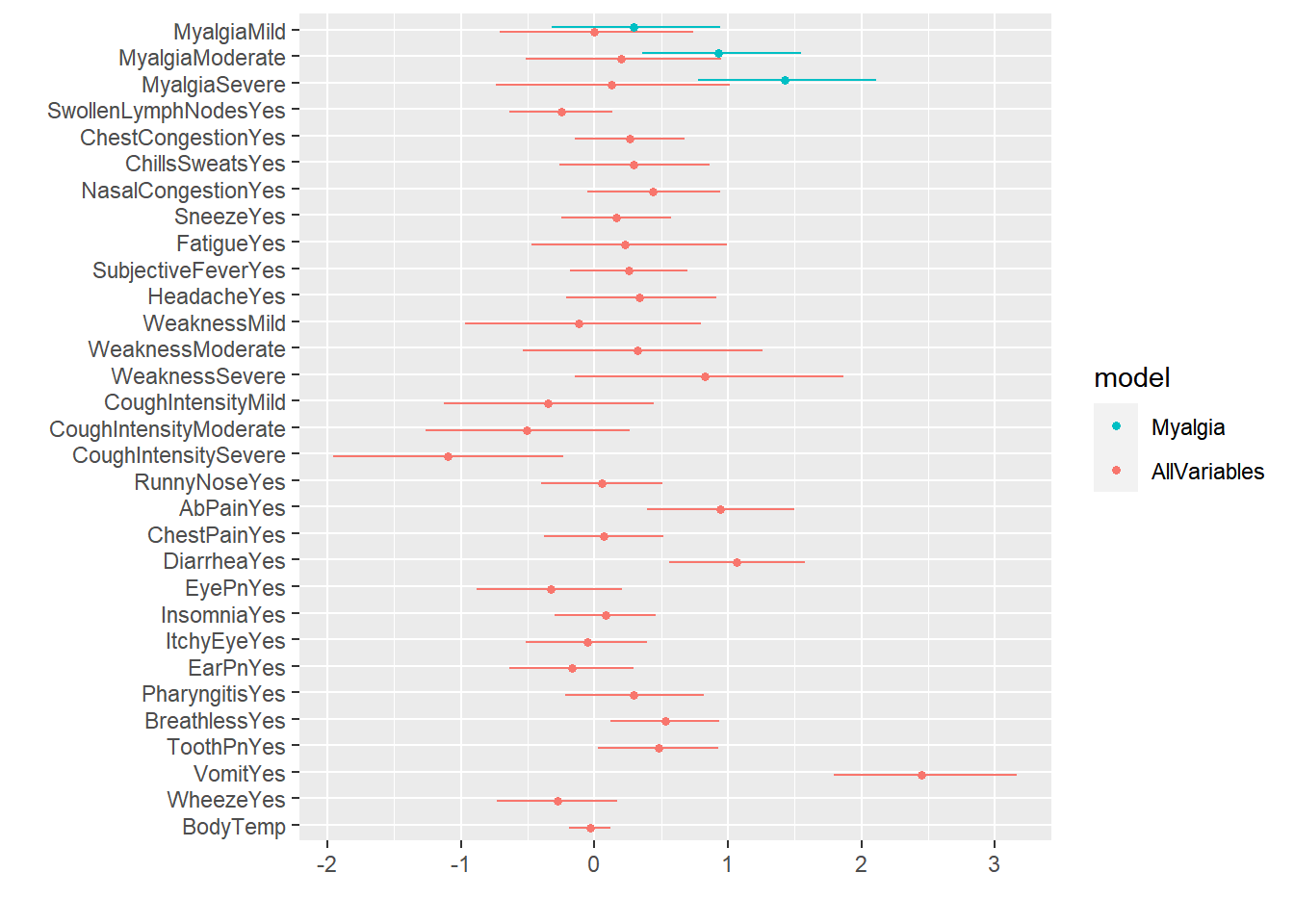
dwplot(list(Myalgia = glm_fit1, AllVariables = glm_fit_all1)) #compare dwplots

glance(glm_fit1) %>%
  dplyr::select( AIC, BIC)
# A tibble: 1 × 2
    AIC   BIC
  <dbl> <dbl>
1  920.  939.
glance(glm_fit_all1) %>%
  dplyr::select( AIC, BIC) #better fit
# A tibble: 1 × 2
    AIC   BIC
  <dbl> <dbl>
1  816.  963.
compare_performance(glm_fit1,glm_fit_all1)
# Comparison of Model Performance Indices

Name         | Model | AIC (weights) | AICc (weights) | BIC (weights) | Tjur's R2 |  RMSE | Sigma | Log_loss | Score_log | Score_spherical |   PCP
--------------------------------------------------------------------------------------------------------------------------------------------------
glm_fit1     |  _glm | 920.3 (<.001) |  920.3 (<.001) | 938.7 (>.999) |     0.044 | 0.466 | 1.121 |    0.625 |  -110.929 |           0.006 | 0.565
glm_fit_all1 |  _glm | 816.1 (>.999) |  819.2 (>.999) | 963.1 (<.001) |     0.246 | 0.415 | 1.038 |    0.515 |      -Inf |           0.002 | 0.657
#Via ANOVA
anova(glm_fit1$fit, glm_fit_all1$fit)
Analysis of Deviance Table

Model 1: Nausea ~ Myalgia
Model 2: Nausea ~ SwollenLymphNodes + ChestCongestion + ChillsSweats + 
    NasalCongestion + Sneeze + Fatigue + SubjectiveFever + Headache + 
    Weakness + CoughIntensity + Myalgia + RunnyNose + AbPain + 
    ChestPain + Diarrhea + EyePn + Insomnia + ItchyEye + EarPn + 
    Pharyngitis + Breathless + ToothPn + Vomit + Wheeze + BodyTemp
  Resid. Df Resid. Dev Df Deviance
1       726     912.28            
2       698     752.13 28   160.15